This article was published in the
C/C++ Users Journal in a two-part
format. The first part of the article appeared in the November 1998 issue,
and the second part in the December 1998 issue.
I hope you find it useful, didactic,
or at the very least, I hope you enjoy reading it. You are free to use the
code presented in this article, being understood that I decline any responsibility,
direct or implied, for damages or inconveniences that its use or impossibility
of use may cause (directly or indirectly). If your local law does not allow
a full decline of responsibility by the author of a software that you use,
then you are not allowed to use the code presented in this article or any
part of it (neither from this web-page, nor downloaded from the C++ Users
Journal web-site).
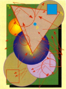
The opening line and the figure appearing
with the title of the article are courtesy of the C++ Users Journal.
If you want to download the entire
code of this article, with a demo and instructions to compile it and run it,
click here.
If you have any comments or question
concerning the content or form, you can reach me by e-mail (visit
my contact page for instructions)
Efficient 2-D Geometric Operations
Carlos Moreno
"Inside"
is an easy predicate for people to determine, but rather harder for
computers.
Introduction
Geometric algorithms and techniques are important tools in Graphics,
Image Processing and Computer Vision applications. They also offer convenient
and efficient solutions to Pattern Recognition problems such as the Nearest
Neighbor rules, Clustering, and Image or Polygons pre-processing.
|
 |
In this article, I present a C++ implementation of some standard and very efficient
algorithms and techniques in the field of Computational Geometry. This implementation
includes fundamental operations such as orientation, test for point inclusion
in a triangle, and segment intersection. These fundamental operations provide
a basis for more complex operations, such as polygon orientation, point inclusion
in a polygon, triangulation, convex hull computation for a set of points and
for a simple polygon, and other standard algorithms.
The tools are based on the implementation of four classes, to represent points,
segments, triangles and polygons, all of them in the plane (two-dimensional).
The Mathematics of 2-D Operations
The basic operation at the heart of the algorithms presented is computation
of a triangle's area given its three vertices (i.e., given the x-y coordinates
of those vertices). This computation is efficiently performed based on the properties
of the vector product.
Given two vectors v1,v2, their vector product v1 x v2 is perpendicular
to both vectors; its magnitude is equal to the product of the magnitudes of
v1 and v2 times the sine of the angle between them; and its orientation can
be obtained using the Right Hand Rule.
If the two vectors are in the x-y plane (i.e., their z-coordinates are zero),
their vector product will be parallel to the z-axis, and its z-coordinate will
be positive if vector v2 is "at the left" of vector v1, zero if v1
and v2 are parallel, and negative if v2 is "at the right" of v1.
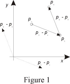
Given three points p1,p2,p3 in the x-y plane, the z-coordinate of the vector
product between p2-p1 (p2 minus p1) and p3-p2 is given by the following formula:
z = x1 (y2 - y3) + x2 (y3 - y1) + x3 (y1 - y2)
|
Given the properties just discussed for the vector product, the above
formula yields the following information (see figure 1):
- The magnitude of z is twice the area of the triangle p1,p2,p3.
- The sign of z tells whether the triplet p1,p2,p3 represents
a right-turn or left-turn (that is, if the point p3 is at the right
or at the left of the oriented segment from p1 to p2)
Notice that only three real number multiplications and five additions
are required to compute this value. No trigonometric function calculations
are involved.
|
|
Surprisingly enough, this simple operation forms the basis of most of the algorithms
that I present in this article, as well as many other extremely complex algorithms.
Even more surprising is the fact that what is (almost exclusively) used in the
algorithms is the sign of Z (i.e., the orientation of triplets of points), rather
than the magnitude or the value itself.
In addition to this fundamental operation and the basic arithmetic (including
the scalar product), two other basic operations (both based exclusively on the
orientation of triplets of points) complete the basis for all the algorithms
that I present: a test for segment intersection, and a test for point inclusion
in a triangle. These two operations are also based exclusively on the orientation
of triplets of points.
Testing for Segment Intersection
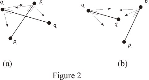
Given two segments (p1,p2) and (q1,q2), they intersect if and only if
the orientation of the triplet (p1,p2,q1) is different from the orientation
of the triplet (p1,p2,q2) and the orientation of the triplet (q1,q2,p1)
is different from the orientation of the triplet (q1,q2,p2). The first
condition means that q1 is on one side of the segment (p1,p2), and q2
is on the other side. The second condition means that p1 is on one side
of the segment (q1,q2), and p2 is on the other side. Clearly, the segments
intersect if and only if both conditions are met, as illustrated in figures
2-a and 2-b.
|
|
Testing for Point Inclusion in a Triangle
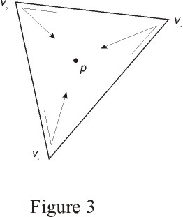
Given a triangle (v1,v2,v3) and a point p, the test for p's
inclusion in the triangle is explained as follows. If we traverse the
points v1,v2,v3 and the point is inside, we will always see the point
on the same side of the segment we are visiting. If v1,v2,v3 are arranged
in a counter-clockwise sense, the points inside it are always at the left
of the segments. If the point is outside, for at least one of the segments
the point will be at the right (see figure 3). If the vertices are arranged
in a clockwise sense, the reasoning is identical, except that a point
that is inside the triangle will always be at the right of the segment
we are visiting.
Thus, to determine if the point p is inside the triangle (v1,v2,v3),
we need only obtain the directions of rotation along the triplets (v1,v2,p),
(v2,v3,p) and (v3,v1,p). The point is inside if and only if the three
directions are equal.
|
 |
A Class to Represent Points
The representation for a point includes a pair of real numbers to store the
x and y coordinates of the point (I use double), as well as member functions
to read each coordinate (get_x and
get_y).
The basic arithmetic operations are provided in the form of overloaded operators.
The arithmetic operations include addition, subtraction, and multiplication
(scalar product). Also, multiplication and division by real numbers is provided
in the form of overloaded operators.
The basic arithmetic operations allow you, for example, to obtain a point that
is inside a triangle given its vertices as follows:
p = (v1 + v2 + v3) / 3;
Also, an overloaded member function is provided to test for inclusion in a
triangle and in a polygon. This allows nice expressions, as shown below:
Point p;
Triangle t;
Polygon P;
if (p.is_inside (t)) // ...
if (p.is_inside (P)) // ...
Similarly, a function to test if a point is exactly on a segment is provided.
This is determined by checking if the segment endpoints (p1,p2) and the point
p are collinear, and if the segments p-p1 and p-p2 have opposite directions
(which means that p is between p1 and p2).
Listings 1-a and 1-b show the code for the class definition and implementation
(respectively) of class Point.
A Class to Represent Segments
The class Segment contains, as data members, two Point objects that represent
a non-oriented segment. (although in most algorithms we deal with it as an oriented
segment from p1 to p2) No operators are provided for this class, since there
are no natural arithmetic operations between segments.
A member function is provided to test for segment intersection. This member
function allows expressions like the following:
Segment s, line;
if (s.intersects (line)) // ...
Listings 2-a and
2-b
show the code for the class interface and implementation of class Segment.
Both Point and Segment classes provide draw member functions.
These member functions are platform dependent. I provide a simplified implementation
for a Win32 platform (without scaling or other considerations). If you want
to use these tools in an application that requires graphical display, you should
provide the implementation for the draw member functions for
Point and Segment.
A Class to Represent Triangles
The class Triangle includes three Point objects representing the vertices of
the triangle. It provides member functions to compute the area and the orientation.
(a private member function is provided to compute the area with sign, which
enables other member functions to obtain the area and the orientation of the
triangle).
Since we are never interested in the exact value of the area of a triangle
(at least not in this type of applications), the member function computes a
value corresponding to twice the area of the triangle, for efficiency reasons.
This may sound crazy, but you'll have to trust me on that one for now (the reasons
should become clear later in this article).
Class Triangle also provides a member function to test if a point is inside
the triangle. This member function allows expressions such as the following:
Triangle t;
Point p;
if (t.contains (p)) // ...
Note that the Point class member function to
test for inclusion is equivalent to this Triangle class operation. The Point's
member function is obviously implemented in terms of this Triangle's member
function (see listing 1-b).
A member function draw is also included. In this case (as with the Polygon
class, yet to be presented), the function is platform independent, since it
is implemented in terms of the Segment class draw member function.
Listings 3-a and
3-b
show the code for the class definition and implementation of class Triangle.
None of the above mentioned classes contains any pointers to dynamically allocated
data or any allocated resources. Therefore, I provide no destructors, copy constructors
or overloaded assignment operators for either of these classes.
A Class to Represent Polygons
A circular doubly-linked list of Points is required to represent a polygon.
The list must be doubly-linked because typical operations on polygons require
insertions and removals of points in the sequence. Some of these operations
must traverse the sequence in reverse, visiting more than one point in succession.
The linked list must be circular because polygons are closed sequences of vertices,
and operations on pairs or triplets of consecutive vertices may not be limited
by the fact that a vertex is the last or the first in the chain.
The implementation of class Polygon uses the STL (Standard Template Library)
list container. For convenience of use, I provide an iterator for this class,
as the standard containers do. Thus, polygons can be manipulated in the same
manner as most of the standard containers, as shown below:
Polygon P;
Polygon::iterator current = P.begin();
do
{
// ...
}
while (++current != P.begin());
Notice that there is no end() member function for
the Polygon container, since it is a circular list.
Also, the typical operations are similar to their equivalents for the standard
containers (e.g., push_back, push_front, insert, remove), which should make
polygon manipulation intuitive to C++ programmers.
No destructor, constructors or assignment operator are required for this class,
since the container included as a data member encapsulates those operations.
Listings 4-a and
4-b
show the definition and implementation of class Polygon and its iterators (class
Polygon::iterator and class
Polygon::const_iterator).
Note that the implementation of these iterators is based on the
list iterator. Their operations are almost a direct
map to the operations of the list iterator, except
for the ++ and -- operators,
since the polygon is a circular list of points.
Geometric Algorithms for Polygons
I will now describe a few algorithms related to polygons, and how I implemented
them in class Polygon. Some of the algorithms are implemented
as member functions, since they correspond to operations inherent to a polygon,
and some are implemented as global functions that use the polygons and their
related operations to perform the processing required.
Unless otherwise specified, polygons are assumed to be simple (i.e., no edges
intersect, and no two vertices are the same point), and, when it is required
to assume an orientation, it will be assumed that the vertices are oriented
in counter-clockwise sense. When dealing with polygons, the term orientation
refers to the apparent sense of rotation when traversing a polygon's vertices.
In particular, if the orientation is counter-clockwise, then the interior of
the polygon will always "touch" the edges on their left. This further
assumes that we are dealing with edges as oriented segments from one vertex
to the next vertex -- i.e., from Vn to Vn+1.
Testing for Point Inclusion in a Polygon
To test if a point p is inside a polygon P, we need find a point that is outside
the polygon, and count how many times the line L from p to the point outside
intersects the polygon. To find a point outside the polygon, we obtain the vertex
with highest x-coordinate and we add one to that x-coordinate.
|
Each time that the line L intersects the polygon, it passes from inside
to outside or vice versa. Thus, if the number of intersections is even,
the point is outside the polygon. If it is odd, the point is inside.
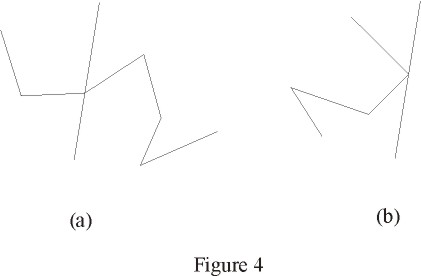
We only need to be careful when the line L passes exactly over a vertex
of the polygon. In that case, we need to check if L intersects the polygon
(figure 4-a) or if it merely touches it (figure 4-b). This is determined
by checking if the segments around the intersecting vertex are on different
sides of L.
Furthermore, if several consecutive vertices
are exactly on the line L, they have to be discarded before checking if
L intersects or touches the polygon. (see
listing 4-b)
|
|
Testing for Polygon Orientation
The orientation of a polygon is often known in advance, since it may be guaranteed
by the mechanism used to obtain the polygon. In some situations, though, we
may have no more at our disposal than a sequence of points, with the knowledge
that it represents a simple polygon. Determining the orientation of such a polygon
consists of three steps:
1) Find a triplet of consecutive vertices such that the triangle formed by
those three vertices does not contain any other vertex of the polygon. If no
other vertex is inside, then the region inside that triangle is either entirely
inside the polygon, or entirely outside the polygon.
2) Determine whether the interior of the triangle found in 1) lies inside or
outside of the polygon. To do this, take any point inside the triangle and test
if it is inside the polygon. If a point inside the triangle is also inside the
polygon, the interior of the triangle lies inside the polygon as well. A point
inside a triangle (p1,p2,p3), is given by (p1+p2+p3) / 3.
3) Determine the orientation of the triplet of
points making up the triangle. If the triplet represents a left turn and the
triangle is inside the polygon, then the polygon is counter-clockwise. Also,
if the triplet represents a right turn and the triangle is outside the polygon,
then the polygon is counter-clockwise. The other two combinations correspond
to a polygon with clockwise orientation (see
listing 4-b).
Finding the Convex Hull of a Simple Polygon
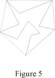
The convex hull of a set R is defined as the smallest (in area) convex
region that contains the entire set R, where R can be a set of points
in the plane, a region, a polygon, the interior of a polygon, etc. If
the set R is a set of points (i.e., a finite number of points) or a polygon,
it can be easily proven that the convex hull is a convex polygon. Figure
5 shows a simple polygon outlined with solid lines, and its convex hull,
in dashed lines.
For an arbitrary set of N points, it has been proven that the convex
hull can not be obtained in less than O(N logN). If the points are known
to form a simple polygon, the scenario is different. For a simple polygon,
several algorithms have been proposed to find the convex hull in linear
time (O(N) operations).
|
|
Most of those algorithms have been proven to be incorrect, including the first
O(N) algorithm proposed, known as the Sklansky scan (also known as the three coins
algorithm), which was accepted and used for several years, until a counter-example
was published, proving that the algorithm would work incorrectly for most arbitrary
polygons.
A detailed discussion about the various convex hull algorithms would be beyond
the scope of this article. I want only to make it clear that the problem is
far more complicated than it looks, despite the simplicity of the algorithm
that I present in this article (the Melkman algorithm).
Melkman proposed an extremely elegant and straightforward algorithm to compute
(in linear time) the convex hull of a simple polygonal chain (which can obviously
be used for a simple polygon). The key idea in this algorithm is to maintain
an updated version of the convex hull, and for each new point encountered in
the input polygonal chain, we test if the convex hull needs to be updated.
The output at any step of the algorithm is a convex polygon with counter-clockwise
orientation, whose first and last elements are the same point, and which correspond
to the last point appended to the output. Thus, the algorithm starts by sending
to the output the first three points of the input polygon (with the appropriate
orientation).
At the step n of the algorithm, we test if the new point (point number n+1
of the input polygon) is outside the convex hull. If it is, then the convex
hull needs to be updated to account for the new point. If not, the new point
is discarded and the output remains the same.
|
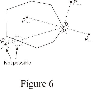
Figure 6 shows an example of the output convex hull, showing the first
two and the last two points, as well as several possibilities of location
for the new point (Pn+1).
Since the algorithm should work in linear time, the test to determine
if the new point is inside the polygon must be done in constant time.
Thus, we cannot use the function previously described to test for point
inclusion in a polygon, since it does not operate in constant time.
In this case, given the way we construct the current convex hull, Melkman
showed a way to determine in constant time if the point is inside the
current convex hull.
If the new point is at the right of the oriented segment P2-P1 and at
the left of the oriented segment Pn-1-Pn, then it is certain that the
point is inside the convex hull, since the line or polyline going from
Pn to Pn+1 (which is part of the input polygon) would have to intersect
the convex hull for the point Pn+1 to be outside. If it intersects the
convex hull, then it intersects the input polygon itself. But since the
input polygon is simple, we know that there are no edge intersections.
|
|
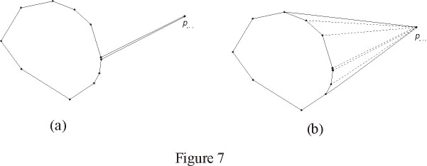
Thus, by testing the orientation for these two triplets of points, we determine
if the new point should be discarded or not. If it is inside, we discard it. If
it is outside, then we append it at both ends of the output, and now we must readjust
the output polygon by removing any vertices that became concave after the insertion
of this new point.
All these updates involve only tests of orientation of triplets of points, since
we know that the output polygon is in counter-clockwise sense, which means that
a left turn represents a convex vertex, and a right turn represents a concave
vertex.
Figure 7 shows an example of this
updating process. Notice that P1 and Pn are actually the same physical point.
In the figure, I show them as two separate points only for illustration
purposes.
|
|
Despite the fact that one step (after O(n) insertions) might involve O(n) removals,
the algorithm does work in linear time (worst-case complexity O(N)). Each point
from the input polygon can be inserted, at most, once into the output, and can
be removed, at most, once. Therefore, we have, at most, 4*N operations (insertions
are done at both ends of the output, and removals may be done from both ends).
Since the test to decide if the point should be discarded is done in constant
time, the algorithm works in linear time.
Listing 4-b shows the details of
the implementation of this algorithm (it is implemented as a member function
that returns a polygon without modifying the object that calls the member function).
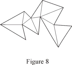
Triangulating a Polygon
Triangulation is an important and very useful operation in many geometry
applications. It provides a representation of a complex figure in simpler
pieces -- triangles.
The result of a triangulation process is a set of triangles for which
each and every vertex can only be a vertex of the polygon being triangulated.
Also, the triangles' internal regions must add up the entire interior
of the polygon. (this is not a formal and rigorous definition of a triangulation,
but you get the idea). Figure 8 shows an example of a polygon and a triangulation
of it. Notice that for a given polygon, the triangulation is not necessarily
unique.
|
|
Some applications require the output of a triangulation to be expressed as
a graph in which adjacent triangles (triangles that share one edge) are adjacent
in the graph. In this article, I restrict the scope of the triangulation algorithm
to provide a non-ordered set of triangles.
The algorithm uses a divide-and-conquer recursive approach, which means that
its expected complexity is N logN. Its worst case complexity, however, is O(N²).
The algorithm requires to know the orientation of the input polygon. Therefore,
counter-clockwise orientation will be assumed. This allows to identify a convex
vertex (when the triplet previous-current-next makes a left turn).
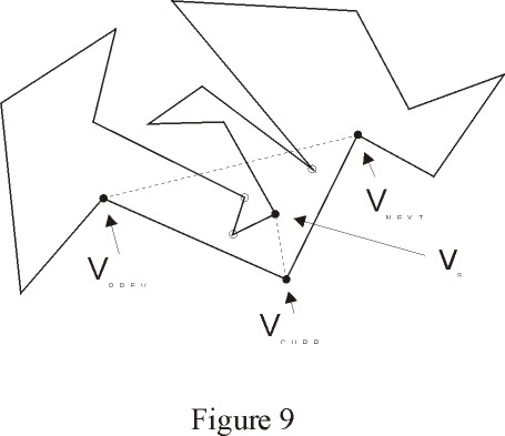
| The algorithm consists of finding convex vertices in the
input polygon. For each convex vertex that we find, we consider the triangle
Vprev-Vcurr-Vnext such that Vprev is the vertex
previous to the convex vertex; Vcurr is the convex vertex;
and Vnext is the point succeding the convex vertex. We now
test if this triangle contains any other vertices of the input polygon.
If the triangle does not contain any other vertex of the input polygon,
then it is guaranteed that the segment Vprev,Vnext does not intersect any
edge of the polygon, therefore, the triangle is sent to the output and the
vertex Vcurr is removed from the polygon. If the triangle does contain other
vertices of the input polygon, we find one of these vertices such that it
can be joined to the vertex Vcurr without intersecting any edges of the
polygon. If we call that vertex Vs, then the segment (Vcurr,Vs) divides
the input polygon into two simple polygons. At this point, we recursively
call the function to triangulate each half of the polygon. (see figure 9)
The stop condition of the recursive process is, of course, when the input
polygon has three vertices (i.e., when it is already a triangle).
|
|
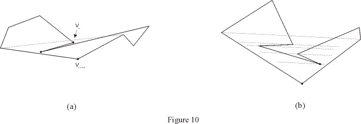
The step of finding a vertex that can be joined to the vertex Vcurr in
the triangle is not as obvious as it looks like. Many wrong approaches have
been used in the past, including the most intuitive, which is finding the
nearest vertex to Vcurr. Figure 10-a illustrates a situation in which this
approach fails, since it produces an output with triangles that intersect
the input polygon. The appropriate way to find such vertex is to find the
point with highest perpendicular distance to the straight line containing
the segment Vprev, Vnext, as illustrated in figure 10-b.
|
|
Naturally, to obtain this point the algorithm does not directly compute a single
distance (it would be too hard, since we are talking about perpendicular distance).
Instead, the algorithm finds the point P for which the area of the triangle
(Vprev,Vnext,P) is maximized. This area is equal to the base (which is fixed,
since it is the distance between Vprev and Vnext) times the height (which is
the perpendicular distance to the base segment) divided by two. Notice that
we don't care that the member function area() actually returns twice the area:
we only want to compare and find the highest area -- the actual value of the
area is of no interest here.
Listing 5
show the code for this triangulation algorithm.
Finding the Convex Hull of an Arbitrary Set of Points
Obviously, an approach to do this in O(N logN) would be to sort the points
by their x-coordinate, which allows us to build a simple polygonal chain (there
can not be edge intersections, since the points are sorted by their x-coordinate)
and now use a linear time algorithm to obtain the convex hull.
A much more straightforward approach, known as the Jarvi's March, is the following:
we first find a point that is on the convex hull (for example, the point with
lowest y coordinate). This can be done in linear time. After that, we find the
right-most point with respect to that first point. The right-most point with
respect to point P is the point X for which no other point of the set is at
the right of the oriented segment from P to X. The right-most point is also
on the convex hull, so we append it to the output and advance. That is, we continue
to find the right-most point with respect to the last point added. We keep going
until the right-most point found is the first point.
Notice that finding the right-most point does not require
any single angle calculation or manipulation -- it can be done by computing
the orientations ofpoint triplets. Listing 6 shows
the code for this algorithm.
Conclusion
Geometric algorithms and techniques are important and convenient tools in many
applications, including Image Processing, Graphics and Pattern Recognition.
Efficiency is in general a very important (maybe the most important) issue,
since applications that involve this type of processing in general act on huge
amounts of information (we may be talking about polygons with several hundreds
or several thousands of vertices). In addition to that, this type of applications
often require real-time processing, with very demanding timing restrictions.
The approach that I presented in this article is based on very efficient mathematical
tools. Most of the operations required for standard geometric algorithms would
not require any single computation of trigonometric functions, square roots,
etc. Instead, a reduced number of multiplications and additions are required
per item processed. In some cases, I sacrificed at some extent efficiency in
exchange for "straightforwardness" of the code. I did this only in
situations where I considered that the impact on the overall speed of execution
is not considerable.
The Object Oriented approach turns out to be extremely appropriate for this
application. Not only is it very intuitive to see geometric entities as software
objects, but also, the approach leads to expressions that are very intuitive
and readable. Also, C++ compilers in general provide very efficient machine
code, which is, as I mentioned before, one of the most important aspects in
this type of applications.
Bibliography
Bjarne Stroustrup. The C++ Programming Language, 3rd Edition.
Addison-Wesley, 1997.
Franco Preparata, Michael I. Shamos. Computational Geometry, An Introduction.
Springer-Verlag, 1985.
Avraham A. Melkman. On-line Construction of the Convex Hull of a Simple Polyline.
Information Processing Letters 25, 1987.